EE3300/EE5300 Electronics Applications Recap of transfer functions and Bode plots
It is assumed that you are familiar with transfer functions from previous study of circuit theory, signals and systems, or similar courses. This section is a quick recap.
The definition of a transfer function
We previously defined the DC gain of an amplifier as the ratio of the output voltage to the input voltage,
We would like to generalise this definition so that it can be used for any arbitrary input signal (such as a sinusoid or some other waveform). You should recall that this type of “gain” equation can be written in the Laplace domain for any linear time-invariant system. Therefore, we define the transfer function as
Notice the direct analogy to Eqs.
Given a Laplace domain transfer function
We can also perform circuit analysis in the Laplace domain using familiar circuit theory techniques (e.g. Ohm’s law, KCL, KVL, node analysis, etc). Laplace domain circuit impedances are shown in Figure 1.
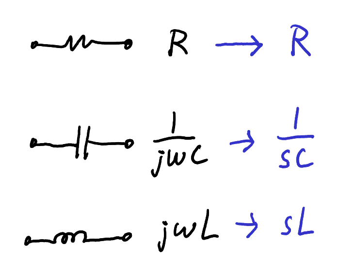
Resistor, capacitor and inductor impedances in the Laplace domain are
Example 1
To refresh our memories about transfer functions, find the transfer function of the low-pass RC filter shown in Figure 2.

A simple RC filter.
Zoom:Solution
We recognise that
It is convenient to write this as
where
Some remarks about this transfer function:
- From Eq.
- Equation
Bode plots
To analyse a circuit’s frequency response, we often use a graphical
tool called a Bode plot. The Bode plot is obtained by substituting
There are simple rules to enable Bode plots to be sketched by hand. It is important to master these rules so that you can intuitively “see” the impact of moving a pole or adding a pole.
We start drawing at low frequencies and progress towards higher frequencies. Each time our sketch passes the frequency of a pole or zero, we change the slope of the magnitude plot. The changes are:
- At each pole: the magnitude plot slope changes by
- At each zero: the magnitude plot slope changes by
For the phase plot:
- At each pole: a total phase shift of
- At each zero: a total phase shift of
Example 2
Sketch the Bode plot of the RC low-pass filter in Figure 2
when
Solution
The DC gain is
There is one pole at
The magnitude plots starts to decrease by
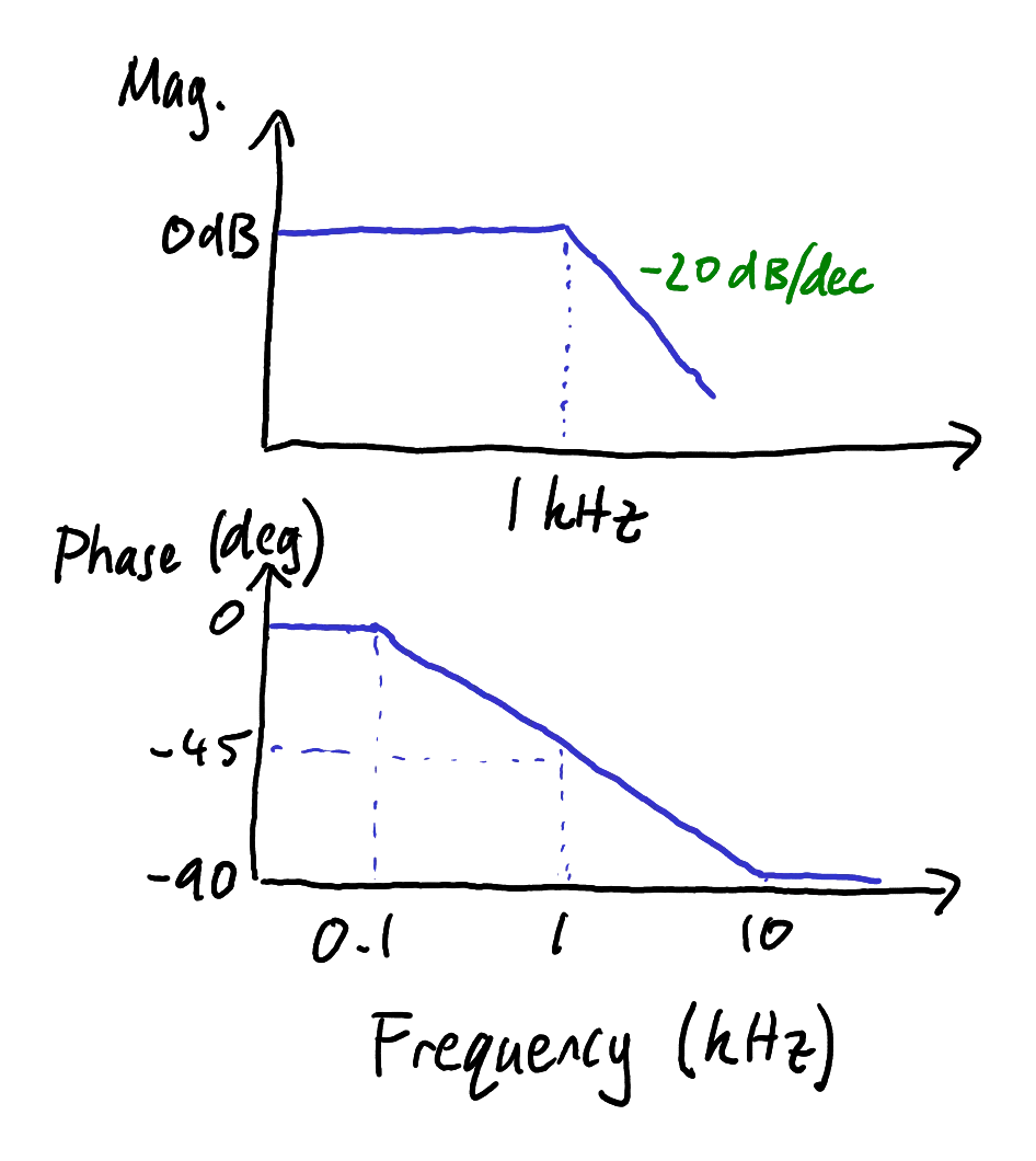
Bode plot hand sketch.
Zoom:For comparison, an accurate plot produced using Matlab’s bode function is shown in Figure 4.

Bode plot produced by Matlab’s bode function.
Show Matlab source code to generate the Bode plot
R = 1e3;
C = 160e-9;
s = tf('s'); % Define the Laplace variable
H = 1/(1 + s*R*C); % Define the transfer function
opts = bodeoptions();
opts.FreqUnits = 'Hz';
opts.XLim = [1e1 1e5];
bodeplot(H, opts);
grid on;