EE3300/EE5300 Electronics Applications Week 3 Practical
Pre-Lab Preparation
In this lab, we explore the concepts of feedback and system stability by analysing op-amp gain and loading, as well as the Colpitts oscillator.
Before the scheduled lab session, perform the following design calculations and simulation tasks.
Part 1: Designing for stability
Recall the requirement for stability: if the loop gain contains sufficient poles to induce a -180° phase shift, the corresponding magnitude must be below 0 dB at this critical frequency. Today we explore how new circuit elements can introduce poles and zeroes and affect stability.
How to measure loop gain in a circuit simulation
Consider the unity gain, non-inverting amplifier configuration in Figure 1. As discussed in the lecture notes, the unity gain case is one of the most difficult to keep stable.

This simple op-amp circuit is surprisingly troublesome for stability.
Zoom:To measure the loop gain in circuit simulation, we must employ some tricks, as shown in Figure 2. We cannot “cut” the loop (as we would in a hand calculation) because then the DC operating point would be lost. Instead, a simple trick is to use a large inductor to effectively cut the loop at AC frequencies while keeping the DC operating point intact.

How to measure the loop gain of the circuit from Figure 1 in LTspice. The AC test signal is capacitively coupled through C1. The enormous inductor L1 isolates the test signal from Vout while permitting DC to pass through.
Zoom:Show more details on loop gain simulations
This simulation is not exact but will give us a close approximation of the loop gain Bode plots. If you would like more information on alternative loop gain simulation methods then please see this video: https://www.youtube.com/watch?v=bXbDa9nglZI.
Draw the circuit of Figure 2 in LTSpice or another simulation program of your choice. Use a generic op-amp model (such as the Universal Op-Amp 5 in LTSpice).
Perform an AC analysis over a large frequency range (e.g. 1 Hz to 1 GHz, with 100 points per decade).
Plot the magnitude and phase of
Hint: In LTSpice, you can customise the equation that is plotted by right clicking on a curve’s title in the plot window. Change the equation to
-V(Vout)/V(Vtest)(adjust as needed based on the node names you have set).👉 Save this plot in your portfolio.
Typical coaxial cable has a capacitance of around 100 pF/m. Suppose you connect approximately 2 m of cable to the output of your circuit, resulting in
Draw the circuit in Figure 3 and repeat steps 2-3.
👉 Save this plot in your portfolio, and predict whether the voltage follower will be stable based upon your observed loop gain.

The modified circuit including a capacitive load.
Zoom:From the loop gain Bode plot, predict the frequency of oscillation by finding the frequency where the phase is -180°. Then perform a transient simulation to check. Save your work to a new circuit file then set it up for transient simulation (as per Figure 4).
Hint: you can determine the frequency of oscillation from the time domain plot by zooming into a region of oscillation, right clicking, selecting View -> FFT, then setting the FFT to be calculated based on the current zoom extent.
👉 Save the transient plot in your portfolio.

The transient simulation setup. The resistor Rf is set to zero to replicate the voltage follower circuit, but in the next section, you’ll increase this value to see the effect of raising the closed-loop gain.
Stability by increasing closed-loop gain
Recall that the closed-loop gain is given by
where
Since the decibel scale is logarithmic (and

The loop gain is the distance between the open-loop gain and the closed-loop gain on a magnitude plot. Raising the closed-loop gain has the effect of decreasing the loop gain.
Zoom:Consider what would happen if we increase our closed-loop gain. This reduces the magnitude of the feedback signal, and hence reduces the magnitude of our loop gain. In this way, by increasing the closed-loop gain of our amplifier circuit, we reduce the loop gain magnitude and effectively force our 0 dB point to occur at a lower frequency. Introducing sufficient closed-loop gain therefore enables us to stabilise our circuit for capacitive loads.
This also explains why the unity-gain case is the most troublesome in terms of stability. We can illustrate this effect in simulation.
Increase the value of
Rfin the circuit from Figure 4 until the circuit is stable.👉 Save the simulation setup and the resulting stable transient plot in your portfolio.
Stability by manipulating the phase margin
A second technique to introduce an isolating series resistor, as we discussed in the lecture notes.
Return the value of
Rfto 0 (so that the circuit again has unity gain).Add a series resistor to the output of the op-amp. Make sure you take the feedback from the correct node, as per the lecture notes.
Adjust the value of the series resistor until the circuit is stable.
👉 Save the simulation setup and the resulting stable transient plot in your portfolio.
Part 2: Designing for oscillation
Sometimes we want a circuit to oscillate! The Colpitts oscillator is a classic example of a circuit that generates a sinusoidal output.
Figure 6 shows a convenient biasing scheme that is ideal for bench prototyping. Here, we use a negative voltage Vee to set the bias point for the transistor. Recall that a BJT’s transconductance is given by
where
Therefore, in a lab setting, adjusting Vee will adjust the bias current, and hence the transconductance of the transistor.

A biasing scheme where a variable voltage supply
Assuming

The Colpitts oscillator circuit.
Zoom:Figure 7 shows a Colpitts oscillator design. Calculate the expected oscillation frequency using the given component values.
Use circuit simulation software (e.g. LTSpice) to perform a transient analysis on this circuit.
Hint: Oscillators are sometimes tricky to get working in simulation because the simulation lacks the thermal noise that would normally kick-start oscillation. One way around this is tell our simulation to skip the initial operating point of the circuit, allowing the simulation to progress into the oscillatory state. Figure 8 illustrates this parameter in a typical LTSpice transient analysis.
Additionally, oscillation can take many cycles to get underway, so you may need to adjust the output start setting to skip over the start-up phase.
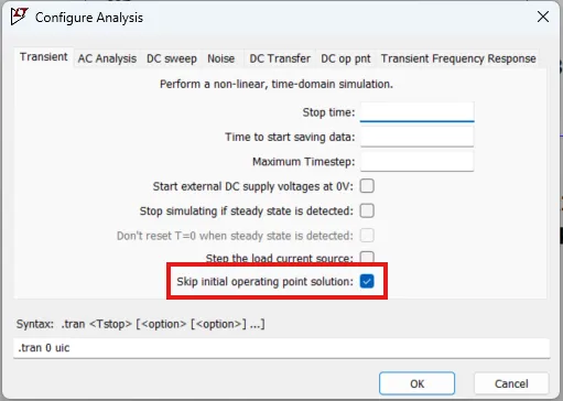
How to tell LTSpice to skip the initial operating point calculation.
Zoom:Experiment with varying the value of
Now plot the emitter voltage
Swap the component values of C1 and C2 (i.e. put the 330 pF capacitor “on top” of the voltage divider and the 1nF capacitor “on the bottom” of the voltage divider). What happens to the distortion? Can you explain why?
How much load can you apply before the oscillator runs into problems?
Hint: How low can
RloadandRloadEbe? These resistors represent the input impedance of the next stage of your circuit, which in real applications may be something like a filter or amplifier circuit (to manipulate your generated sinusoidal wave).
👉 Save your results in your portfolio.
Equipment
- 1x LF411 JFET Input Op-Amp.
- 2x Female BNC Breadboard connectors.
- 1x 2m Coaxial male-to-male cable.
- 2x Breadboards (one for the main circuit and one for the downstream ‘load’ stage).
- 1x 10k Potentiometer.
- 1x SFH 2505 Photodiode.
- 1x 2N3904 NPN BJT.
- 1x 33uH inductor.
- 1x LED (any colour).
- Various capacitors.
- Various resistors.
Instructions to students
These activities require you to compare step responses of various circuits. You should save oscilloscope screenshots to your portfolio as you go, making note of exactly what circuit you were testing at the time.
- Work individually on these activities.
- Focus on neat circuit breadboarding.
- Include power supply decoupling capacitors.
- Use ceramic (non-polar) capacitors for the Colpitts oscillator circuit.
Exercise 1: Putting a signal into a coax cable: what could possibly go wrong?
In this exercise, we will see that introducing even a small, seemingly benign capacitance to a closed feedback loop can be enough to push an otherwise stable circuit into instability.
Your task is to observe the stability and signal quality effects of driving a load through a relatively short length of coaxial cable.
Construct the left side of the circuit in Figure 9.

The circuit to be constructed in the lab.
Zoom:Test that your follower (not yet connected to any load) is working. Drive your circuit with a 1 kHz 3 V square wave and measure the output. Make sure that your driver circuit is behaving as expected.
👉 Save an oscilloscope screenshot (showing the input and output signals on separate channels) in your portfolio.
Construct a second breadboard with a small load resistor (150 Ω) as per the right side of Figure 9. This will represent our external system. You might think of this as an external sensor or actuator we are trying to control with our central processor. Use BNC connectors to connect the coaxial cable to your breadboards.
Connect your two circuit boards with 2-3 m of coaxial cable.
Measure the output waveform of your amplifier and compare against the input square wave. What do you notice about the output?
Stability effects caused by capacitive loads can be a bit unpredictable. You should see some ringing or oscillations that corrupt the square wave output. However, if your voltage follower produces a beautiful clean square wave without any issue, then you can add some capacitance across the load. The extra capacitance is essentially faking the case of having a longer length of coax cable.
👉 Save your oscilloscope traces in your portfolio.
Exercise 2: Exploring stability compensation
Your task is to experimentally demonstrate the stability compensation techniques we explored in the pre-lab simulations, first by adjusting the closed-loop gain (magnitude manipulation), then by introducing an isolating resistor (phase manipulation).
Modify your circuit from Exercise 1 to include a 10 kΩ potentiometer as shown in Figure 10.

Coax driver with variable gain using a potentiometer.
Zoom:What effect does the introduction of this potentiometer have on your circuit? What do you notice as you vary the potentiometer value? Are you able to affect the stability of the circuit?
👉 Document your findings in your portfolio.
Try disconnecting the load resistor (so that the coax end is open-circuit) and repeating this process.
👉 Document your findings in your portfolio.
Replace the potentiometer with a series resistor, as per Figure 11. Do you notice any stability improvements? Try some higher resistance values.
👉 Document your findings in your portfolio.

Coax driver with isolating resistor.
Zoom:Exercise 3: Constructing a transimpedance amplifier
We’ve explored the stability effects of capacitive loads in the seemingly straightforward case of a coaxial cable. What happens if the capacitance is introduced on the input side instead?
Your task is to construct a transimpedance amplifier to interface with a photodiode light sensor. You will then modify the circuit to ensure stability.

The transimpedance amplifier circuit.
Zoom:Construct the transimpedance amplifier circuit as shown in Figure 12.
Hint: You can use the diode test mode on your multimeter to help you orient the photodiode. The datasheet may not be particularly helpful here. Alternatively, looking into the diode head, the cathode (flat part of the diode schematic) is usually the larger side (connected to the main diode body). If you orient your diode incorrectly, your output voltage polarity will be reversed.
Observe the output of your op-amp with an oscilloscope as you cover the photodiode and/or shine a torch light over it. You should see a change in output voltage that relates to the light intensity that appears on the photodiode.
Use an LED to test the step response of the photodiode. Use a function generator to drive the LED with a square wave. Experiment to find the correct voltage to drive the LED (start low and gradually increase it).
Position the LED close to the photodiode. You should see some oscillatory behaviour in the output of the amplifier.
👉 Document your findings in your portfolio.

The transimpedance amplifier with a compensating capacitor.
Zoom:Review the circuit in Figure 13. C1 is an unwanted parasitic capacitance due to the photodiode. A typical value for this capacitance can be found in the photodiode’s datasheet. It should be clear to you that the parasitic capacitance will introduce a pole into the circuit.
👉 Determine an expression for the pole frequency in terms of
Hint: draw the circuit with the input stimulus turned off, notice that the output of the op-amp becomes 0 V, simplify the circuit, and use the technique from the week 2 lecture notes to find the pole frequency.
Now calculate the frequency of the zero. Notice that the response through the feedback network is zero at the frequency where
👉 Write down your expression in your portfolio.
Using Figure 11 in the lecture notes as a guide, choose an appropriate value for
Show optional step: how to use Matlab for more accurate analysis
Figure 11 in the notes has limited options for the pole and zero frequency.
You can use the Matlab script below to generate plots for arbitrary pole and zero frequencies.
Rf = 100e3;
Ci = % insert your value here
Cf = % insert your value here

f_pole = 1/(2*pi*...); % insert your expression here
f_zero = 1/(2*pi*...); % insert your expression here

% op-amp transfer function
s = tf('s');
A_OL = 1e5; % open loop gain at low frequencies
f_op_amp_pole = 50; % read this from its datasheet plot of open-loop gain
A = A_OL / (1 + s/(2*pi*f_op_amp_pole));

% feedback network transfer function
B = (1 + s/(2*pi*f_zero)) / (1 + s/(2*pi*f_pole));

% plot the loop gain and step response
figure();
bodeplot(A*B);
figure();
step(A / (1 + A*B));
Add your chosen value of
👉 Save oscilloscope screenshots showing the change in step response with and without the compensation capacitor.
Exercise 4: Constructing a Colpitts oscillator
Your final activity this week is to build a circuit that is deliberately designed to oscillate.
The Colpitts oscillator circuit (Figure 7 repeated here for convenience).
Zoom:Construct the Colpitts oscillator circuit as shown in Figure 14.
Use an oscilloscope to observe
👉 Save oscilloscope screenshots.
Calculate new values for the Colpitts tank circuit to increase the oscillating frequency above 3 MHz.
Hint: There are multiple ways to achieve this outcome. Consider which of the components will physically be easiest to change. Ensure you consider the relative magnitudes of your capacitors to avoid the effects highlighted in your pre-lab simulations.
Modify the circuit to change the oscillation frequency and test your new design. Have you achieved your aim of oscillation above 3 MHz frequency?
👉 Save oscilloscope screenshots demonstrating the new frequency of oscillation.
Portfolio template
Instructions: copy and paste the following template into a document. Answer each question as you work through the practical. Use that document when you ask to be marked off for this practical. You also need to include these results as part of your final portfolio submission at the end of the study period.
Simulation of loop gain without load capacitance
Show the simulation setup and the Bode plot for the loop gain. Based on this plot, determine the phase margin.
Simulation of loop gain with load capacitance
Show the Bode plot for the loop gain. Answer these questions: Is this circuit stable and why/why not? Based on the Bode plot, estimate the frequencies of the poles. Predict the frequency of oscillation by finding the frequency where the phase is -180°.
Transient simulation
Show the transient simulation and check your earlier prediction of the oscillation frequency.
Improving stability by two techniques
Show your circuit and resulting transient simulation when you make the circuit stable by increasing the gain and when you introduce a series resistor.
Simulations of the Colpitts oscillator
Show the circuit and transient simulations under different conditions with varying capacitor values and loads, as discussed in the instructions.
Exercise 1: Voltage follower driving a capacitive load
Include screenshots showing the behaviour of your follower when driving no load and when driving the load through the coax cable. Comment on each case and explain the results.
Exercise 2: Improving stability by two techniques
Include screenshots showing the behaviour of your driver circuit when the gain is adjusted and when there is a series resistor. Comment on each case and explain the results.
Exercise 3: Transimpedance amplifier
Show the step response of the transimpedance amplifier circuit when the light turns on and off.
Write down your expressions for the pole and zero frequencies, and hence find a suitable value for the compensation capacitor Cf.
Show how the step response improves when the compensation capacitor is added.
Exercise 4: Colpitts oscillator
Show the initial circuit design and your modification(s) to increase the frequency, including measurements of the output waveforms.
Conclusion
Your tutor will mark you off for completing this activity and being able to discuss the results. If you do not finish on time, bring your completed portfolio to a subsequent lab session for marking.
When you leave, make sure that the lab is just as neat or even neater than when you arrived.
References
This activity was adapted from Lab 9 in Learning the Art of Electronics by Hayes and Horowitz. Some other material was derived from Solving Op Amp Stability Issues by Green and Wells of Texas Instruments.