EE3901/EE5901 Sensor Technologies
Chapter 1 Tutorial

Written by A/Prof Bronson Philippa and Laurance Papale

College of Science and Engineering, James Cook University

Last updated 21 February 2025

Question 1

A potentiometer is being used as a displacement sensor. It has the transfer function plotted in Figure Q1.

(a) Over what range of displacements is this sensor linear?

(b) Determine the sensitivity in the linear region.

(d) You measure using a multimeter that shows two digits after the decimal point, i.e. the multimeter gives readings like 2.21 V and 2.22 V. What is the resolution of this overall system, assuming that you are using the sensor in its linear region?

Answer

(a) The sensor is linear within the range of 0 mm - 2 mm (approximately). The deviation from linearity appears to start just before 2 mm but it is difficult to judge by eye.

(b) The sensitivity is 0.4 V/mm. This is obtained from the slope of the transfer function.

where is measured in volts and is the displacement in mm.

(d) The voltage resolution (the smallest change that can be detected) is 0.01 V. We can convert this to mm by using the sensitivity as a conversion factor. By dimensional analysis,

Question 2

An accelerometer has a measurement range of where is the acceleration due to gravity. The measurement is digitally sampled and represented as a 12-bit signed integer. Assume that the response is linear across the entire measurement range.

(a) What is the sensitivity of this sensor system?

(b) What is the resolution of this sensor system?

(c) By repeatedly sampling the same acceleration, it is found that the measurement noise can be described by a Gaussian distribution whose standard deviation is equal to 4.4 counts in the integer scale of the accelerometer. Convert this to acceleration in units of g.

(d) When the sensor is sitting on the lab bench it is measuring an acceleration of 1 g. Given the noise characteristics of part (c), what is the signal-to-noise ratio?

Answer

(a) The full span is . Meanwhile the full span output covers digital states. In other words the least significant bit (LSB) of the output can change times when sweeping across the entire measurement span. Since we are told that the system is linear, the slope of the transfer function must be:

(b) For digital systems, the resolution is always the reciprocal of the sensitivity.

(d) Use the factor of 20 in the signal to noise ratio calculation because we are measuring signal amplitude (not power).

Question 3

Suppose that an integrated pressure sensor receives dual power supply rails ( V). However, the transfer function specified by the manufacturer indicates that the output voltage depends upon the value of the positive supply rail :

where is the input pressure in kPa and is the positive supply voltage in V. The supply voltage is normally 5.0 V.

The sensor has a measurement range of 0 to 250 kPa.

(a) Find the sensitivity.

(b) Suppose that an inexperienced engineer did not read the entire sensor datasheet and did not find the actual transfer function, Eq. . Instead, they found a table of performance characteristics that included the sensitivity you calculated in part (a). Based on the sensitivity, they guessed a transfer function of the form

where is sensitivity and is pressure.

The sensor is outputting a voltage of 3.7 V. What is the error in pressure that will result from the use of the incorrect transfer function?

The prototype device has insufficient voltage regulation, and the supply voltage sometimes drops from the normal 5.0 V down to a minimum of 4.85 V. Unfortunately this variation in the supply voltage is not accounted for. In the transfer function the incorrect value continues to be used.

What is the worst case absolute error in the measured pressure caused by this unstable power supply?

Hint: solve the transfer function for the measurement . This will enable you to explore what happens to the apparent pressure when varies. You will need to algebraically rearrange to find an expression for the measurement error .

Answer

(a) Sensitivity = 0.02 V/kPa.

(b) The hapless engineer uses their incorrect transfer function to obtain the formula

Meanwhile from the true transfer function we obtain

Hence the error is

Next consider the actual when the supply voltage drops:

Substituting,

We want to find the error . For this, we need on the LHS, so we expand 0.97 into 1 - 0.03 and bring to the other side:

By sketching this function (Figure A3) or by analysing its functional form, we can see that the worst case error will occur at the maximum of the measurement range at kPa. Therefore the worst case absolute error is

Question 4

You are testing an actively powered light sensor that measures light intensity and responds with an electrical current. Your device is rated for a maximum light power of . You are testing your device by exposing it to different intensities of light from a calibrated source, and you measure the electrical power that is dissipated when the sensor’s output current is passed through a 50 Ω resistor. The resulting measurements are shown in Figure Q4.

Figure Q4:
Measurement results for Question 4.
Zoom:

(a) Estimate the dynamic range of this sensor.

(b) What is the SNR for an input power of ?

Answer

(a) DR = 40 dB. You can read this directly from the graph by noticing that there are 4 decades between the noise floor and the maximum output power (since the graph covers the full span of the sensor).

(b) SNR = 20 dB. Note that you need to convert from input power to output power in order to compare against the noise floor. Again you can visually see 2 decades which is 20 dB.

Question 5

Figure Q5:
An illustration of “accuracy” (bias) vs precision. Image by Byron Inouye.
Zoom: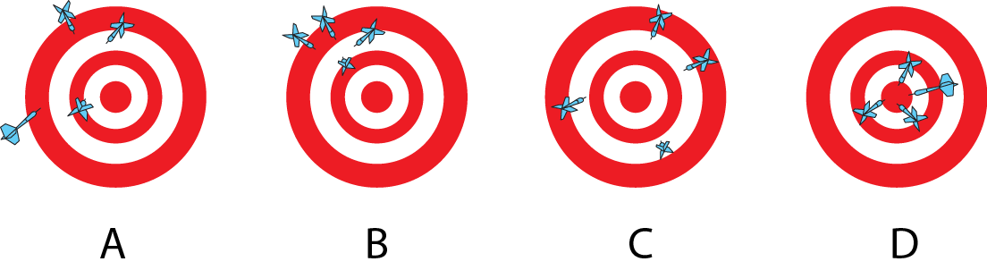

A dart board can be used to illustrate the difference between accuracy and precision, where accuracy in this case means bias. Assume that the goal is for all darts to hit the bullseye in the centre of the board.

(a) Rank these boards in order from most accurate to least accurate.

(b) Rank these boards in order from most precise to least precise.

Answer

(a) Cases C and D are the most accurate but it’s difficult to visually determine which is the more accurate of the two. They are approximately equally accurate since the average of all throws is close to the centre. Cases A and B are similar. Hence the ranking from most to least accurate would be: (C and D tied), (A and B tied).

(b) The ranking from most precise to least precise would be: D, B, A, C.

(c) Accuracy (bias) can be determined by measuring reference values that are known through other means. Precision can be determined by measuring the same value repeatedly and studying the noise characteristics.

Question 6

A tachometer is an instrument that measures rotational speed. Suppose that you are working with a tachometer that is mechanically coupled to a shaft and acts as an AC generator by producing a sinusoidal voltage in time with the rotations of the shaft. The tachometer is a 2 pole alternator, i.e. its electrical frequency matches the shaft rotational frequency. The tachometer is an AC voltage source with Ω of output resistance (Figure Q6.1). The tachometer is connected to a servo motor control system with an input resistance of Ω. The servo motor system measures the frequency of the AC voltage at in order to determine the rotational speed of the shaft.

Figure Q6.1:
Circuit diagram showing the tachometer equivalent circuit connected to the motor controller equivalent circuit.
Zoom:

The output voltage of the tachometer is shown in Figure Q6.2.

(a) Notice that the voltage is reduced from the tachometer’s open circuit voltage due to the input impedance of the motor controller. Calculate the relative error in the voltage due to this electrical loading.

(b) In part (a), we treated the tachometer as a resistive device. However in reality its windings are inductive. If included an inductive component, would the error become smaller, stay the same, or increase when the shaft’s rotational speed varies?

(c) Suppose that the windings of the tachometer have an inductance of 50 mH, i.e. is changed to 10 Ω + 50 mH. The servo motor control system requires a minimum RMS voltage of = 1.0 V in order to reliably detect the signal. What is the highest shaft speed that can be measured by this sensor system?

(d) What is the dynamic range of this system?

Answer

(a) Using the voltage divider rule, the output voltage is

The relative error is

Here the ideal value (in the absence of the electrical loading of ) would be simply . Therefore,

Hence, the relative error is -4%.

(b) The sensor output impedance is , and a faster shaft speed means a larger , which means larger , hence worse voltage drop. The relative error will become larger (more negative).

From Figure Q6.2, the open circuit voltage V at high speeds. Therefore,

The question states that we must have V. Hence, we must solve for frequency in the expression

This frequency has units of radians/second. The frequency in hertz is

Use dimensional analysis to figure out the conversion ratio from Hz to rpm. We want units of “per minute” whereas we currently have “per second”.

Therefore the maximum shaft speed is 49,472 rpm.

(d) The dynamic range is defined to be

The maximum value (from part c) is 49472 rpm. The minimum value can be determined from Figure Q6.2. Recall that the minimum voltage must be 1 V. This occurs at 100 rpm. You could simply use 100 rpm directly from the graph (ignoring the electrical loading of the motor controller), in which case you could calculate a dynamic range of

However, a better answer would account for the electrical loading. You could observe that the low end of Figure Q6.2 has a slope of 1 V per 100 rpm. Therefore you can write

where is the open circuit voltage of the tachometer and is the shaft speed in rpm. At these low speeds, the impedance of the inductor will be negligible. Therefore, using your result from part (a),

Using the minimum voltage requirement,

This gives a dynamic range of

Question 7

Let and be random variables that have variances and respectively. Let be a scalar function. If and are uncorrelated then prove that the standard deviation of is

Hint: write expressions for the Jacobian and covariance matrix and then use .

Answer

Since and are uncorrelated, the covariance matrix has zeros in the off-diagonal positions. Hence

Therefore

Question 8

You measure the current flowing through a circuit element and obtain mA, where the uncertainty is interpreted as the standard deviation of the measurement. Next, you measure the resistance of this element and obtain Ω, again where the uncertainty is interpreted as the standard deviation of the measurement. You believe that the current and resistance error are uncorrelated.

What is the voltage across the circuit element () and its associated uncertainty?

Hint: use Eq. (1), above.

Answer

Question 9

A thermistor (a temperature sensor) has a transfer function

where is the resistance, is the absolute temperature, is the resistance at a temperature and is a sensitivity constant.

(a) Suppose that there is a measurement uncertainty in , modelled by a standard deviation . Assuming that all other parameters are exact, find an expression for the standard deviation in temperature.

(b) Now suppose that the uncertainty is instead found in the parameter . All other parameters are exact but has a standard deviation . Find an expression for the standard deviation in temperature.

(c) Now suppose that both and are subject to uncertainty. You may assume that the two parameters are uncorrelated. Find an expression for standard deviation in temperature.

(d) If you change to a different thermistor with increased sensitivity (i.e. larger value of ), but keep everything else the same, would you expect the temperature precision to change?

Answer

(a) .

(b) .

(d) Yes, a more sensitive thermistor will result in less variance in temperature. Intuitively, the more the resistance changes, the easier it is to characterise the underlying temperature because the spread of resistances corresponds to a smaller spread of temperatures. (If you cannot see this, draw the transfer function with two different slopes and imagine the impact of a given amount of resistance error.)

Question 10

A robot uses a wheel encoder to measure its velocity. There is software running on the robot that numerically differentiates velocity to obtain acceleration. The errors in velocity and acceleration are correlated because they derive from the same physical sensor.

The power consumption of the robot is estimated using the formula

where the first term represents drag and the second term represents the force required to change the acceleration.

When the robot is maintaining a constant velocity, the standard deviation of the velocity measurement is found to be . Later, a constant acceleration is applied, and the standard deviation of the acceleration measurement is found to be . The correlation in the errors is .

At a given instant, the measurements are and . What is the standard deviation in ?

Answer

Question 11

A wearable inertial measurement unit is being used to monitor curvature of the spine during rowing. The sensor (Figure Q5) has a flat edge that is taped to the participant at specific vertebra of the spine. The parameter of interest is flexion and extension of the spine, meaning how far the person has bent forward or backward. This is characterised by the angle of the sensor with respect to the vertical, i.e. 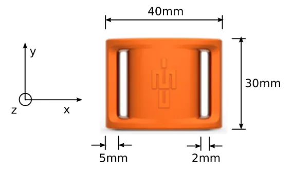the angle between the sensor axis and the vertical direction in the lab’s reference frame.

Figure Q11:
The sensor being considered in this question. Image from Vicon IMeasureU BlueThunder data sheet.
Zoom:

The angle can be calculated using the formula

where and are the respective components of a unit vector that express the sensor’s Y axis in the reference frame of the laboratory.

Calculate the standard deviation in given the following parameters:

Hint: the derivative of arctan (when the angle is expressed in radians) is

Answer

Given we have

Hence the Jacobian is

The covariance matrix is

Hence the standard deviation of is

Question 12

A linear actuator drives a terminal device (e.g. gripper, hand, etc) of a robotic manipulator. The force exerted by the gripper is related to the displacement of the linear actuator by a function . For example, imagine a spring where the force depends upon how tightly it is compressed. However, the actual may be different to that of a spring. The system is designed such that and across the entire range of motion.

Figure Q12:
The relationship between the linear actuator and terminal device.
Zoom:

The terminal device is known to be perfectly accurate, but there is some error in the linear actuator. The error is expressed as a percentage by normalising to the standard deviation, e.g.

and

(a) Show that the relative error in the force is given by:

(b) Find a suitable transfer function such that the force error remains constant across the entire range of motion.

Hint: If the force error is constant then it must have no dependence upon f or x. Write an equation, separate the variables to obtain on one side and on the other side, then integrate and solve for .

Answer

(a) Outline of proof: use the result

and use the definitions of and to eliminate and respectively. Also use the fact that standard deviations are always positive so you can take the positive square root only when simplifying the equation.

(b)

where a is an arbitrary constant.

Question 13

You are calibrating a low-cost temperature sensor using the one point calibration method. With the sensor on the laboratory bench, you measure the temperature five times and obtain the following results: 26.86 °C, 26.91 °C, 28.04 °C, 27.99 °C, 27.99 °C.

You also have a reference thermometer, which you believe is substantially more accurate than the cheap sensor you are calibrating. It gives you the following measurements: 24.91 °C, 25.21 °C, 25.05 °C, 24.99 °C, 25.05 °C.

(a) Calculate the expected value of the measurements according to the sensor and the reference thermometer.

(b) Calculate the standard deviation of the measurements according to the sensor and the reference thermometer.

(d) Calibrate the cheap sensor, i.e. obtain an expression that can be used to correct for the bias.

(e) Suppose that you decide to combine information from both sensors by averaging their measurements. In other words, you will take both sensors into an environment to measure, you will obtain two measurements, and then average the result. Repeating 5 times as in the example here, you obtain a total of 10 measurements. What is the standard deviation obtained using this method?

(f) You notice from part (e) that the standard deviation of the average is worse than the standard deviation of just using the better sensor, i.e. there was no benefit obtained from the cheap sensor at all. Intuitively, there must be one way to extract information even from low quality sensors, so you are motivated to try a weighted average method of the form

where , is the measurement according to the cheap sensor, and is the measurement from the better sensor. Find a value for that minimises , and the value of at this minimum value.

Note: this principle (of giving more weight to those measurements which have lower variance) is a key concept behind the Kalman filter, which you will study in Week 2.

Answer

(a) °C; °C.

(b) °C; °C.

Note that you must use the sample estimator, i.e.

with the on the denominator because this is just a sample, not the entire population.

(d) °C.

(e) Assuming uncorrelated errors, °C.

(f)

The standard deviation of the combined measurement is

i.e. smaller than the result in part (b). This shows that there was a benefit in combining the information from both sensors.