EE3901/EE5901 Sensor Technologies Chapter 3 NotesResistive sensors
In this chapter we introduce resistance as a physical mechanism for sensing and circuit designs used to interface with resistive sensors.
Introduction to resistive sensors
A resistive sensor is a device whose electrical resistance varies in response to changes in the measurand.
We will examine several types of resistive sensors in this chapter.
Potentiometers
A potentiometer is a device for measuring linear or rotary displacement. Examples are shown in Figure 1.
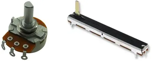
Example rotary (left) and linear (right) potentiometers. (Images from element14).
Zoom:Potentiometers have a sliding contact, called a wiper, that moves along a resistive element (Figure 2). The wiper makes contact at a point

(a) The circuit symbol is three terminal device showing the resistor and wiper. (b) The impact of the wiper is to split the resistance into two parts connected in series.
Zoom:There are rotary and linear potentiometers. For rotary potentiometers, there are single-turn and multi-turn devices. Multi-turn potentiometers place the resistive element in a helical shape so multiple turns are needed to fully traverse its length.
Potentiometers are cheap, robust, and can be quite accurate. The resistance between wiper and terminal is ideally proportional to the displacement being measured. In practice there are some inaccuracies that prevent this assumption from being perfectly true.
Limitations
The resistance will not be perfectly uniform along its length. This limits the linearity of the potentiometer. Furthermore, many potentiometers are made with coiled wire, so there will be step changes as the sliding contact touches each new coil during its movement. Typical deviations from linearity are in the range of 0.002% FSO to 0.1% FSO (full scale output).
The resistance changes with temperature. If the temperature variation across the element is uniform then the effect on the output voltage will cancel out. However if there is non-uniform heating (e.g. because of power dissipation inside the potentiometer) then temperature effects will have an impact.
Some other practical concerns:
- Potentiometers have a power rating, which will limit the maximum applied voltage and also minimum input impedance that the wiper can be connected to.
- The friction and inertia of the wiper add mechanical load to the system being measured. Potentiometers are best used to measure relatively slow movements.
Strain gauges
A strain gauge is a thin foil of conductive material that is glued or otherwise attached to a mechanical element in order to measure its deformation. Strain gauges use the principle of piezoresistivity, which is the change in resistance due to mechanical deformation (strain).

An example scenario where a strain gauge could be applied. The cantilevered beam bends under the influence of the force, which is detected by the strain gauge.
Zoom:A simple use of a strain gauge is shown Figure 3. As a mass is applied, the beam will bend, stretching out the strain gauge and hence changing its resistance. This effect is called piezoresistivity.
Piezoresistivity

A length of wire is stretched by an axial force. The piezoresistive effect is the resulting change in resistance.
Zoom:Consider a conductive wire with a given resistance. Now imagine that the wire is stretched out so that it becomes longer and thinner, as shown in Figure 4. What will be the resulting change in resistance?
To develop a theory of piezoresistivity, first we need to understand the concepts of stress and strain.
Stress is the amount of force applied per unit area. Specifically,
where
Stress causes some deformation in the material that is called “strain”. Strain is the dimensionless change in length
where
As shown in Figure 5, materials typically have an “elastic region” where there is a linear relationship between stress and strain, and the material recovers if the stress is removed. Beyond that point there is permanent deformation and eventual breakage of the material.

Typical relationship between stress and strain. Our strain gauges will operate in the elastic region, where there is a neat linear relationship between the two quantities. (Figure adapted from Pallas-Areny & Webster, 2001).
Zoom:The relationship between stress and strain in the elastic zone is given by Hooke’s law
where
Returning the wire being stretched, the electrical resistance is given by
where
where
Using strain gauges on structural elements
Applying a stress to a wire by itself is not very common; in practice we often want to measure the strain on some structural or mechanical element. Hence the idea of a strain gauge is to attach a piezoresistive sensor to the mechanical element. In that way the strain in the mechanical element also affects the sensing element. Both deform together, but the strain in the sensor is measured electrically.
Example 5.1
A strain gauge has an unstressed resistance of
Solution
The strut will experience a strain of
The resulting change in resistance is
Hence we have
Notice how this is quite a small change in resistance, so a carefully designed interfacing circuit will be needed. In this case a good design is called a Wheatstone Bridge, and we will study it soon.
Optimising the strain gauge
Compared with metals, semiconductors often display a much larger piezoresistive effect. Changes in inter-atom spacing affects the semiconductor band gap, resulting in changes to the concentration of charge carriers as well as their mobility. Gauge factors for semiconductors are typically in the range of about 40 to 200.
A strain gauge will typically arrange the piezoresistive element to maximise sensitivity in one direction while minimising sensitivity in the other. This is achieved with long thin segments in the sensing direction and wide segments in the non-sensing direction (Figure 6).
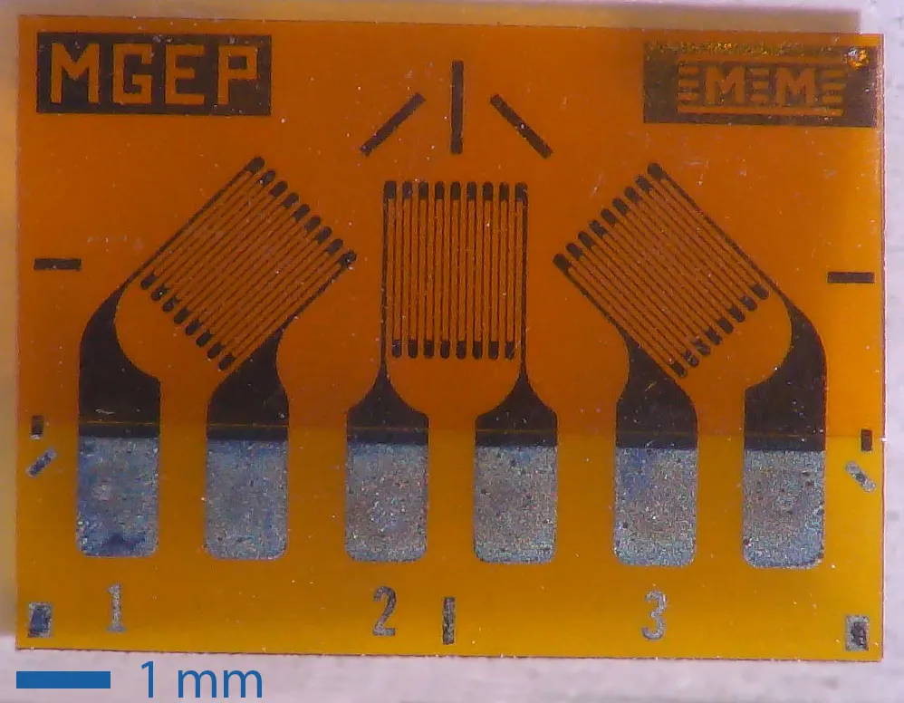
Optical microscope image of a device that includes 3 strain gauges. Each gauge is sensitive to flex along the directions indicated by the short dark lines at the top of the image.
Zoom:Practical issues with strain gauges
- The strain must be mechanically transmitted to the gauge, i.e. it must be properly affixed to the element being monitored.
- The applied stress must not exceed the elastic limit of the gauge, which is typically in the range of 3000 με for semiconductor gauges and 50,000 με for metal gauges.
- Temperature interferes with strain gauge measurements by influencing the materials’ resistivity, dimensions, and the Young’s modulus of the support material. Change in temperature leads to a change in resistance, and hence a change in apparent strain. A typical method to compensate is to provide additional strain gauges that not subject to any strain. The ‘dummy gauges’ should experience the same temperature changes, and hence can be used to compensate for changes in resistance.
Resistive temperature detectors (RTDs)
The resistance of a material changes with temperature. An RTD is a device that uses this mechanism for sensing. Typically RTDs have a polynomial response of the form
where
For RTDs, the most common material to use is platinum, in which case the device is sometimes called a PRT (platinum resistance thermometer). Other metals used include copper, nickel and molybdenum.
Sometimes temperature dependence is characterised by the temperature coefficient of resistance (TCR), which gives the proportion change in resistance for a given change in temperature.
Example 5.2
A copper conductor has a resistance of
Answer
so we have
Temperature measurements based on resistance need special care because
resistance can only be measured by passing a current through the element.
The applied current will heat up the sensor, disturbing the measurement.
This effect can be characterised by a heat dissipation constant
where
Example 5.3
A given PRT has a heat dissipation constant of
Answer
The goal is to maintain
The major advantages of RTDs are:
- High sensitivity (ten times higher than thermocouples)
- High repeatability
- Long-term stability
- Wide span (i.e. -200 C to 850 C for platinum)
Thermistors
A thermistor is another type of thermally sensitive resistor. In contrast to the metals used in RTDs, thermistors are based on semiconductors. The typical operating mechanism is that increased temperature excites more charge carriers into the conduction band, and hence decreases the resistance. Such devices are called negative temperature coefficient (NTC) thermistors. However, other thermistors exhibit the opposite behaviour of having a positive temperature coefficient (PTC).
Thermistor transfer functions are non-linear. An approximation is the the “B parameter equation”
where
This model is only useful over a small span, so a more accurate transfer function is the Steinhart-Hart equation
The coefficients
Thermistors are less stable than RTDs but otherwise have similar properties. The measurement span for thermistors is smaller than RTDs.
Applying a current through a thermistor will cause it to heat up. This effect can be an issue for temperature measurements. However, some applications rely upon thermistor self-heating. Examples of these applications are shown in Figure 7.

Example circuits showing the self-heating mechanism of a negative temperature coefficient (NTC) thermistor. (a) The temperature of the thermistor can rise when it is out of the liquid. As it heats, its resistance drops. Eventually the current is high enough to activate the relay and pump more liquid into the tank. The liquid cools the thermistor, deactivating the relay. (b) The thermistor takes time to heat up, thereby implementing a time delay between the closing of the switch and the activation of the relay coil. (Figure adapted from Pallas-Areny & Webster, 2001).
Zoom:The circuit in Figure 7a controls the level of liquid in a tank. When the liquid is low, the thermistor self-heats until its resistance is small. A small resistance then permits enough current to flow to activate the relay coil and engage the pump.
The circuit in Figure 7b provides a time-delayed start. When the thermistor is cold, its resistance is high enough that the relay cannot activate. As the thermistor self-heats, its resistance drops, and then sufficient current flows to activate the relay coil.
Conversely, PTC thermistors can be used to provide current-limiting effects, e.g. as a self-resetting “fuse” where a high current causes the temperature to rise to the point where the resistance becomes large enough to effectively shut off the circuit. Once the fault is cleared, the thermistor cools down and its resistance drops.
Photoresistors (light dependent resistors)
A light dependent resistor (LDR), also called a photocell or photoresistor, is a device where the resistance declines in the presence of light. These devices are made from semiconductors. Incident light excites charge carriers into the conduction band, hence increasing the conductivity of the device. The most common materials for LDRs are CdS, CdSe, PbS, and PbSe, each of which is sensitive to different wavelengths of light. However, these materials are restricted by Europe’s RoHS (reduction of hazardous substances) regulations, and hence photoresistors are becoming less common.
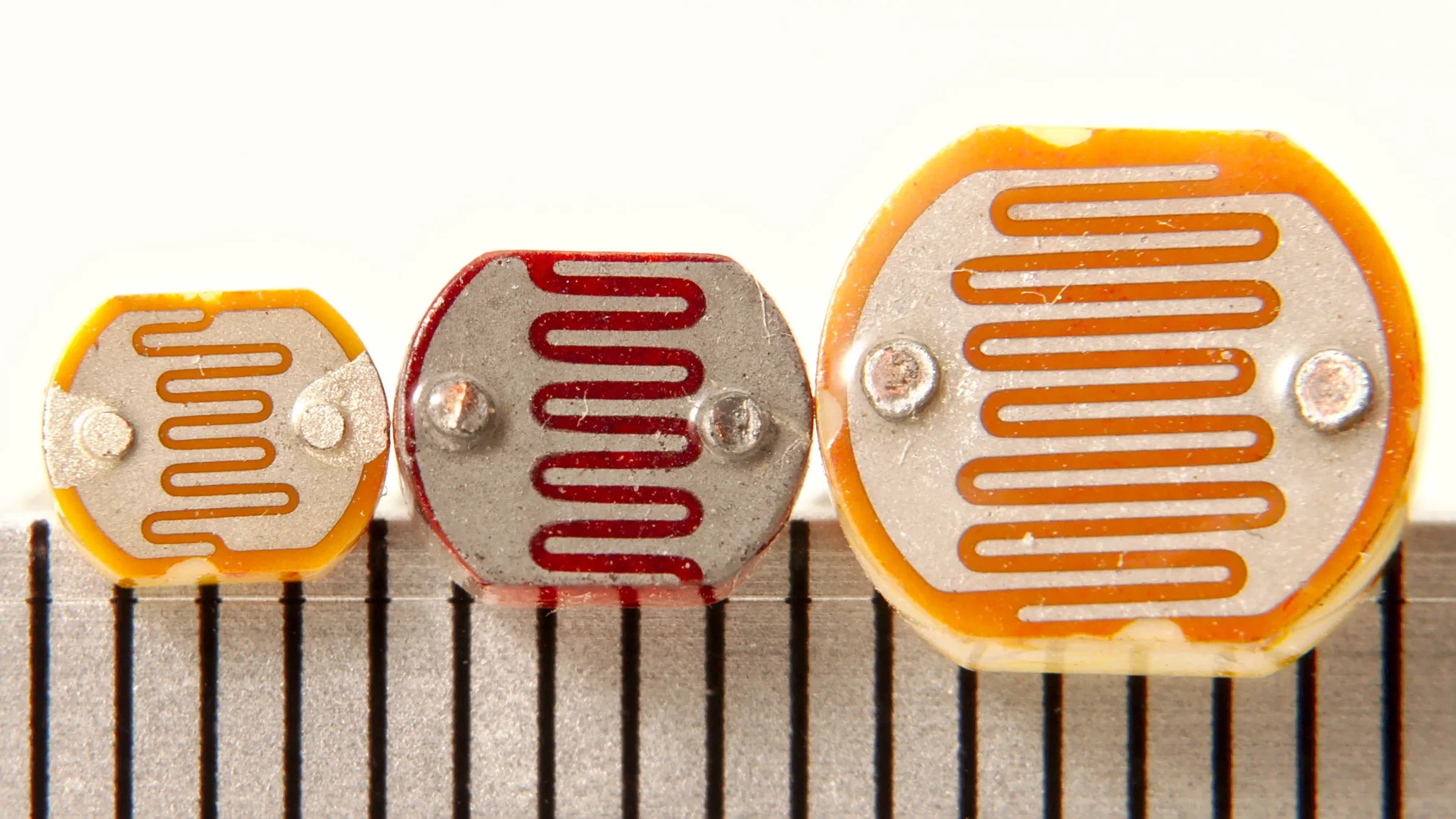
Examples of photoresistors, with a scale bar in millimeters. (Image credit: By Junkyardsparkle - Own work, CC0, https://commons.wikimedia.org/w/index.php?curid=35977178).
Zoom:Photoresistors typically have fairly slow response times (e.g. 10s of milliseconds) so they are mostly suitable for measuring constant levels of brightness.
Interfacing with resistive sensors
There are two requirements for all resistive sensor interface circuits:
- The circuit must drive the resistive sensor with a voltage or current. Resistance can only be measured when there is a current flowing.
- The voltage and current must be low enough to avoid self-heating of the sensor (unless self-heating is part of the operational mechanism of the sensor, in which the interface circuit must ensure appropriate levels of power dissipation).
The two wire measurement circuit
The simplest approach is to measure resistance with Ohm’s law. Apply a current and measure the voltage, or vice versa. A typical circuit is shown in Figure 9.

The two wire measurement circuit. Here
The weakness of this approach is that the resistance of the cabling will affect the measurement. The cable resistance will vary with temperature so it not always easy to correct for. Hence, the two wire approach is generally unsuitable for precision measurements.
The four wire measurement circuit
A better design separates the voltage measurement from the excitation current, as shown in Figure 10.

The four wire measurement circuit, where
If the voltmeter has a large input impedance, then the sensing current
Measuring small changes in resistance
Suppose that we want to measure small changes in a large resistance. For example, imagine we have a sensor whose resistance changes from 10,000 Ω to 10,001 Ω. How can we design circuits to interface with such a sensor?
To formalise the problem, consider a sensor with a transfer function of the form
where
An example of such a circuit is the Wheatstone Bridge.
The Wheatstone Bridge Circuit
A Wheatstone Bridge is two voltage dividers in parallel. It is often drawn in a diamond shape, like Figure 11.

The concept of a Wheatstone bridge.
Zoom:There are two main ways to use the Wheatstone Bridge. These are called “balance mode” and “deflection mode”.
Balance mode
In balance mode, a current meter is connected across the bridge, as shown in Figure 12.

A Wheatstone bridge wired in balance mode.
Zoom:Resistor
The user adjusts
Deflection mode
The second way to use the Wheatstone Bridge is in “deflection mode” where a voltage meter is connected across the bridge:

A Wheatstone bridge in deflection mode.
Zoom:Analysing this circuit, the output voltage is
The Wheatstone Bridge is typically used with strain gauges or RTDs
where a small change in resistance must be detected. Let
where
Designing a bridge circuit is then a matter of choosing
Using the Wheatstone Bridge with strain gauges
A common configuration is to place multiple strain gauges in a single bridge circuit. The configurations are called “quarter bridge” (one sensor), “half bridge” (two sensors) and “full bridge” (four sensors).
The half bridge
If the gauges measure equal but opposite strains, connect each sensor to the same side of the half bridge, as per Figure 14.

A half bridge circuit. The strain gauges on opposite sides of the beam are connected on the same arm of the Wheatstone bridge.
Zoom:Analysing this circuit, we find
Simplifying,
Notice how the output voltage does not depend upon
The full bridge
The full bridge circuit is shown in Figure 15.

A full bridge circuit. Strain gauges with equal responses are placed at diagonally opposite sides of the bridge.
Zoom:Here the output voltage is
Notice that this is twice as sensitive as the half bridge.
Differential amplifiers
The voltages obtained from a Wheatstone Bridge are measured between two nodes in the circuit. For many applications we need to amplify the signal and convert it to a “single ended” voltage measured with respect to ground (for example, to connect to a microcontroller’s ADC). In other words, we want something of the form
where
Your first year circuits textbook probably shows you an op-amp circuit that appears to solve this problem, most likely with something like Figure 16. However, there are some practical issues with this circuit that need to be explained.

Don’t do this. It is a circuit design that works in theory but will not succeed in practice, as discussed in the text. Use an instrumentation amplifier instead.
Zoom:Let’s first analyse this circuit to see how it’s supposed to work. Assuming the op-amp is operating within its linear regime, some elementary circuit analysis will show you that the output voltage is given by
Since we want an output proportional to
Solving for the input voltages:
Substituting into
where the common mode gain is
and the differential mode gain is
To use this circuit as a differential amplifier we require
A desirable parameter for a differential amplifier is to have a high common mode rejection ratio (CMRR), defined as
There will some CMRR due to the tolerance of the resistors, as well as some CMRR due to the op-amp itself.
A further problem with this circuit is the input impedance. The resistors
need to be in the range of 10s to 100s of kΩ for good op-amp performance.
However, the resulting input impedance looking into
Instrumentation Amplifiers
An instrumentation amplifier (sometimes called an “in-amp”) is an IC that solves the problems of a basic op-amp differential amplifier. It has excellent CMRR and extremely high input impedance.
The basic design of an instrumentation amplifier is shown in Figure 17.

The simplified equivalent circuit of an instrumentation amplifier. The highlighted region is manufactured in a single integrated circuit, allowing for precise trimming of the matching resistors so that the tolerate problems mentioned in the previous section can be avoided.
Zoom:You should be able to recognise two voltage followers and the differential
amplifier stage from earlier. Notice how the input impedance looking
into
The output voltage is
where
Often all components except for
Conclusion
In these notes, we have surveyed some common types of resistive sensors. These are:
- potentiometers (for measuring linear or angular displacement),
- strain gauges (for measuring mechanical loads),
- resistive temperature detectors and thermistors (for measuring temperature), and
- photoresistors (for measuring light intensity).
Naturally, there are many other types of resistive sensor that you are likely to encounter. In this week’s practical, you will design and build a circuit using an instrumentation amplifier. Specifically, you will use the Texas Instruments INA826. Please refer to that device’s datasheet to familiarise yourself with its properties.
References
Ramon Pallas-Areny and John G. Webster, Sensors and Signal Conditioning, 2nd edition, Wiley, 2001.
Winncy Y. Du, Resistive, Capacitive, Inductive, and Magnetic Sensor Technologies, CRC Press, 2015.