EE3901/EE5901 Sensor Technologies
Week 5 Notes
Resistive sensors

Written by Dr. Bronson Philippa

College of Science and Engineering, James Cook University

Last updated: 21 March 2023

This week we introduce resistance as a physical mechanism for sensing.

Introduction to resistive sensors
Potentiometers
- Limitations
Strain gauges
Resistive temperature detectors (RTDs)
Thermistors
Photoresistors (light dependent resistors)
Conclusion
References

Introduction to resistive sensors

A resistive sensor is a device whose electrical resistance varies in response to changes in the measurand.

We will examine several types of resistive sensors in this chapter.

Potentiometers

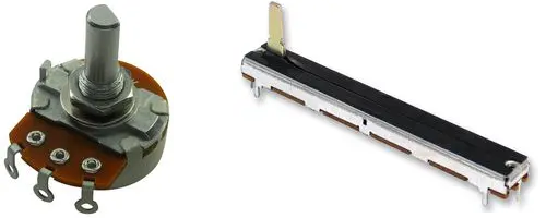
A potentiometer is a device for measuring linear or rotary displacement. Examples are shown in Figure 1.

Potentiometers have a sliding contact, called a wiper, that moves along a resistive element (Figure 2). The wiper makes contact at a point $x$ along the resistor. If the resistor is of length $L$ then it is effectively split into two parts in proportion to the fraction $\alpha = x/L$ .

Figure 2: (a) The circuit symbol is three terminal device showing the resistor and wiper. (b) The impact of the wiper is to split the resistance into two parts connected in series. Zoom:

There are rotary and linear potentiometers. For rotary potentiometers, there are single-turn and multi-turn devices. Multi-turn potentiometers place the resistive element in a helical shape so multiple turns are needed to fully traverse its length.

Potentiometers are cheap, robust, and can be quite accurate. The resistance between wiper and terminal is ideally proportional to the displacement being measured. In practice there are some inaccuracies that prevent this assumption from being perfectly true.

Limitations

The resistance will not be perfectly uniform along its length. This limits the linearity of the potentiometer. Furthermore, many potentiometers are made with coiled wire, so there will be step changes as the sliding contact touches each new coil during its movement. Typical deviations from linearity are in the range of 0.002% FSO to 0.1% FSO (full scale output).

The resistance changes with temperature. If the temperature variation across the element is uniform then the effect on the output voltage will cancel out. However if there is non-uniform heating (e.g. because of power dissipation inside the potentiometer) then temperature effects will have an impact.

Some other practical concerns:

Potentiometers have a power rating, which will limit the maximum applied voltage and also minimum input impedance that the wiper can be connected to.
The friction and inertia of the wiper add mechanical load to the system being measured. Potentiometers are best used to measure relatively slow movements.

Strain gauges

A strain gauge is a thin foil of conductive material that is glued or otherwise attached to a mechanical element in order to measure its deformation. Strain gauges use the principle of piezoresistivity, which is the change in resistance due to mechanical deformation (strain).

Figure 3: An example scenario where a strain gauge could be applied. The cantilevered beam bends under the influence of the force, which is detected by the strain gauge. Zoom:

A simple use of a strain gauge is shown Figure 3. As a mass is applied, the beam will bend, stretching out the strain gauge and hence changing its resistance. This effect is called piezoresistivity.

Piezoresistivity

Figure 4: A length of wire is stretched by an axial force. The piezoresistive effect is the resulting change in resistance. Zoom:

Consider a conductive wire with a given resistance. Now imagine that the wire is stretched out so that it becomes longer and thinner, as shown in Figure 4. What will be the resulting change in resistance?

To develop a theory of piezoresistivity, first we need to understand the concepts of stress and strain.

Stress is the amount of force applied per unit area. Specifically,

\begin{equation} \sigma=\frac{F}{A}, \end{equation}

where $\sigma$ is stress (in units of $\text{N}/\text{m}^{2}$ ), $F$ is the force, and $A$ is the cross-sectional area.

Stress causes some deformation in the material that is called “strain”. Strain is the dimensionless change in length

\begin{equation} \epsilon=\frac{\Delta L}{L}, \end{equation}

where $\Delta L$ is the change in length and $L$ is the original (unstressed) length. The strain $\epsilon$ is dimensionless, but is sometimes written as m/m to indicate meter of deformation per meter of length. Sometimes you will see strain given in units of microstrains where 1 microstrain = 1 με = $10^{-6}$ m/m.

As shown in Figure 5, materials typically have an “elastic region” where there is a linear relationship between stress and strain, and the material recovers if the stress is removed. Beyond that point there is permanent deformation and eventual breakage of the material.

Figure 5: Typical relationship between stress and strain. Our strain gauges will operate in the elastic region, where there is a neat linear relationship between the two quantities. (Figure adapted from Pallas-Areny & Webster, 2001). Zoom:

The relationship between stress and strain in the elastic zone is given by Hooke’s law

\begin{equation} \sigma=E\epsilon \end{equation}

where $E$ is the Young’s modulus. The Young’s modulus is a property of a given material.

Returning the wire being stretched, the electrical resistance is given by

\begin{equation} R=\frac{\rho L}{A} \end{equation}

where $\rho$ is the resistivity of the material from which the wire is made. When stress is applied, the length will increase according to Hooke’s law, and also the cross-sectional area will shrink. Together these effects combine to increase the resistance. There is a relationship

\begin{equation} \frac{\Delta R}{R}=G\frac{\Delta L}{L}=G\epsilon \end{equation}

where $G$ is the “gauge factor” of the material. Gauge factors for metals are typically in the range of 2 - 5. This change in resistance due to stress is called the piezoresistive effect. The piezoresistive effect in metals is typically driven by changes in geometry.

Using strain gauges on structural elements

Applying a stress to a wire by itself is not very common; in practice we often want to measure the strain on some structural or mechanical element. Hence the idea of a strain gauge is to attach a piezoresistive sensor to the mechanical element. In that way the strain in the mechanical element also affects the sensing element. Both deform together, but the strain in the sensor is measured electrically.

Example 5.1

A strain gauge has an unstressed resistance of $R=350$ Ω and a gauge factor of $G=2.1$ . It is glued to an aluminium strut with a cross-sectional area of 191 $\text{mm}^{2}$ . Aluminium has a Young’s modulus $E=73$ gPa. What is the change in the strain gauge resistance when the strut supports a 1000 kg load?

Solution

The strut will experience a strain of

\epsilon=\frac{\sigma}{E}=\frac{F}{AE}=\frac{1000\times9.8}{\left(191\times10^{-6}\right)\times\left(73\times10^{9}\right)}=7.029\times10^{-4}=702.9\ \text{με}.

The resulting change in resistance is

\frac{\Delta R}{R}=G\epsilon=2.1\times7.029\times10^{-4}=0.00148.

Hence we have

\Delta R=350\times0.00148=0.52\ \text{Ω}.

Notice how this is quite a small change in resistance, so a carefully designed interfacing circuit will be needed. In this case a good design is called a Wheatstone Bridge, and we will study it next week.

Optimising the strain gauge

Compared with metals, semiconductors often display a much larger piezoresistive effect. Changes in inter-atom spacing affects the semiconductor band gap, resulting in changes to the concentration of charge carriers as well as their mobility. Gauge factors for semiconductors are typically in the range of about 40 to 200.

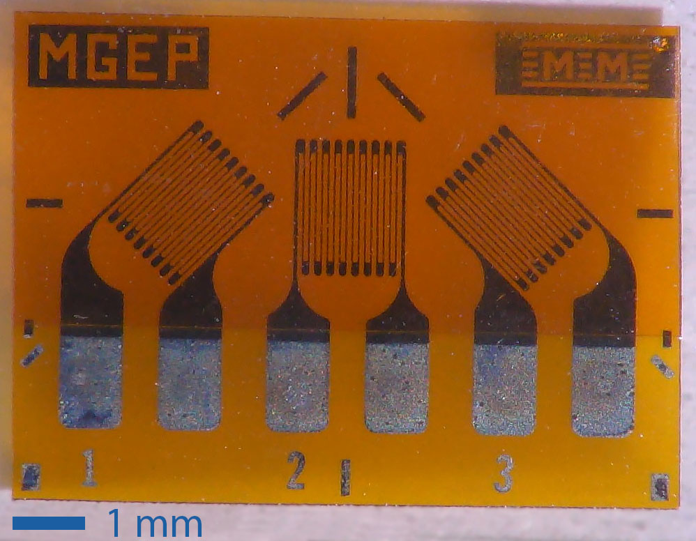
A strain gauge will typically arrange the piezoresistive element to maximise sensitivity in one direction while minimising sensitivity in the other. This is achieved with long thin segments in the sensing direction and wide segments in the non-sensing direction (Figure 6).

Figure 6: Optical microscope image of a device that includes 3 strain gauges. Each gauge is sensitive to flex along the directions indicated by the short dark lines at the top of the image. Zoom:

Practical issues with strain gauges

The strain must be mechanically transmitted to the gauge, i.e. it must be properly affixed to the element being monitored.
The applied stress must not exceed the elastic limit of the gauge, which is typically in the range of 3000 με for semiconductor gauges and 50,000 με for metal gauges.
Temperature interferes with strain gauge measurements by influencing the materials’ resistivity, dimensions, and the Young’s modulus of the support material. Change in temperature leads to a change in resistance, and hence a change in apparent strain. A typical method to compensate is to provide additional strain gauges that not subject to any strain. The ‘dummy gauges’ should experience the same temperature changes, and hence can be used to compensate for changes in resistance.

Resistive temperature detectors (RTDs)

The resistance of a material changes with temperature. An RTD is a device that uses this mechanism for sensing. Typically RTDs have a polynomial response of the form

\begin{equation} R(T)=R_{0}\left[1+\alpha_{1}\left(T-T_{0}\right)+\alpha_{2}\left(T-T_{0}\right)^{2}+\cdots\right] \end{equation}

where $R$ is the resistance at temperature $T$ , $R_{0}$ is the resistance at a reference temperature $T_{0}$ , and $\alpha_{1}$ , $\alpha_{2}$ , … are calibration coefficients. Typically $\alpha_{2}$ and higher are small, so the response is close to linear.

For RTDs, the most common material to use is platinum, in which case the device is sometimes called a PRT (platinum resistance thermometer). Other metals used include copper, nickel and molybdenum.

Sometimes temperature dependence is characterised by the temperature coefficient of resistance (TCR), which gives the proportion change in resistance for a given change in temperature.

\begin{equation} \text{TCR}=\frac{\left(\frac{dR}{dT}\right)}{R}\approx\alpha_{1}. \end{equation}

Example 5.2

A copper conductor has a resistance of $25$ Ω at 25 °C. Given that copper has a TCR of 0.0039 $\text{K}^{-1}$ , what will be the resistance at 100 °C?

Answer

\frac{\Delta R}{R}=0.0039\times75=0.2925

so we have $\Delta R=0.2925\times25=7.3$ Ω. The new resistance is $R+\Delta R=32.3$ Ω.

Temperature measurements based on resistance need special care because resistance can only be measured by passing a current through the element. The applied current will heat up the sensor, disturbing the measurement. This effect can be characterised by a heat dissipation constant $\delta$ (in units of W/K), i.e. the RTD will heat up by an amount

\begin{equation} \Delta T=\frac{P_{D}}{\delta} \end{equation}

where $P_{D}$ is the power dissipated in the RTD.

Example 5.3

A given PRT has a heat dissipation constant of $\delta=100\ \text{mW}/\text{K}$ . If the device has a resistance of $100$ Ω, calculate the maximum allowable sensing current to keep the self-heating error $\Delta T$ below 0.1 K.

Answer

The goal is to maintain $\Delta T<0.1$ . The dissipated power is $P_{D}=I^{2}R=100I^{2}$ . Substituting into Eq. (3),

\begin{align*} \Delta T & <0.1\\ \frac{P_{D}}{\delta} & <0.1\\ \frac{100I^{2}}{0.1} & <0.1\\ I^{2} & <10^{-4}\\ I & <0.01\ \text{A}. \end{align*}

The major advantages of RTDs are:

High sensitivity (ten times higher than thermocouples)
High repeatability
Long-term stability
Wide span (i.e. -200 C to 850 C for platinum)

Thermistors

A thermistor is another type of thermally sensitive resistor. In contrast to the metals used in RTDs, thermistors are based on semiconductors. The typical operating mechanism is that increased temperature excites more charge carriers into the conduction band, and hence decreases the resistance. Such devices are called negative temperature coefficient (NTC) thermistors. However, other thermistors exhibit the opposite behaviour of having a positive temperature coefficient (PTC).

Thermistor transfer functions are non-linear. An approximation is the the “B parameter equation”

\begin{equation} R=R_{0}\exp\left(B\left[\frac{1}{T}-\frac{1}{T_{0}}\right]\right) \end{equation}

where $R_{0}$ is the resistance at temperature $T_{0}$ and $B$ is a sensitivity coefficient. This equation can be rearranged to yield

\begin{equation} \frac{1}{T}=\frac{1}{T_{0}}+\frac{1}{B}\ln\left(\frac{R}{R_{0}}\right). \end{equation}

This model is only useful over a small span, so a more accurate transfer function is the Steinhart-Hart equation

\begin{equation} \frac{1}{T}=a+b\ln R+c\left(\ln R\right)^{3}. \end{equation}

The coefficients $a$ , $b$ and $c$ need to be obtained by calibration.

Thermistors are less stable than RTDs but otherwise have similar properties. The measurement span for thermistors is smaller than RTDs.

Applying a current through a thermistor will cause it to heat up. This effect can be an issue for temperature measurements. However, some applications rely upon thermistor self-heating. Examples of these applications are shown in Figure 7.

Figure 7: Example circuits showing the self-heating mechanism of a negative temperature coefficient (NTC) thermistor. (a) The temperature of the thermistor can rise when it is out of the liquid. As it heats, its resistance drops. Eventually the current is high enough to activate the relay and pump more liquid into the tank. The liquid cools the thermistor, deactivating the relay. (b) The thermistor takes time to heat up, thereby implementing a time delay between the closing of the switch and the activation of the relay coil. (Figure adapted from Pallas-Areny & Webster, 2001). Zoom:

The circuit in Figure 7a controls the level of liquid in a tank. When the liquid is low, the thermistor self-heats until its resistance is small. A small resistance then permits enough current to flow to activate the relay coil and engage the pump.

The circuit in Figure 7b provides a time-delayed start. When the thermistor is cold, its resistance is high enough that the relay cannot activate. As the thermistor self-heats, its resistance drops, and then sufficient current flows to activate the relay coil.

Conversely, PTC thermistors can be used to provide current-limiting effects, e.g. as a self-resetting “fuse” where a high current causes the temperature to rise to the point where the resistance becomes large enough to effectively shut off the circuit. Once the fault is cleared, the thermistor cools down and its resistance drops.

Photoresistors (light dependent resistors)

A light dependent resistor (LDR), also called a photocell or photoresistor, is a device where the resistance declines in the presence of light. These devices are made from semiconductors. Incident light excites charge carriers into the conduction band, hence increasing the conductivity of the device. The most common materials for LDRs are CdS, CdSe, PbS, and PbSe, each of which is sensitive to different wavelengths of light. However, these materials are restricted by Europe’s RoHS (reduction of hazardous substances) regulations, and hence photoresistors are becoming less common.

Figure 8: Examples of photoresistors, with a scale bar in millimeters. (Image credit: By Junkyardsparkle - Own work, CC0, https://commons.wikimedia.org/w/index.php?curid=35977178). Zoom:

Photoresistors typically have fairly slow response times (e.g. 10s of milliseconds) so they are mostly suitable for measuring constant levels of brightness.

Conclusion

In these notes, we have surveyed some common types of resistive sensors. These are:

potentiometers (for measuring linear or angular displacement),
strain gauges (for measuring mechanical loads),
resistive temperature detectors and thermistors (for measuring temperature), and
photoresistors (for measuring light intensity).

Naturally, there are many other types of resistive sensor that you are likely to encounter.

Next week, we will discuss how to design interface circuits to connect resistive sensors to the rest of your electronics.

References

Ramon Pallas-Areny and John G. Webster, Sensors and Signal Conditioning, 2nd edition, Wiley, 2001.

Winncy Y. Du, Resistive, Capacitive, Inductive, and Magnetic Sensor Technologies, CRC Press, 2015.