EE3901/EE5901 Sensor Technologies

Week 7 Notes

Capacitive sensors and signal conditioning circuits for reactive sensors

Capacitance

Firstly, let’s review the physics of capacitors. A capacitor consists of two electrodes separated by an insulating material. An accumulation of charge on the electrodes creates an electric field between the plates. The electric field causes the effects we know as capacitance.

Capacitance is measured in farads (F), which is equivalent to coulombs/volt. In other words the capacitance tells you how much electric charge will accumulate on each electrode per volt.

Suppose we have rectangular electrodes, as shown in Figure 1.

These are called “plane parallel” electrodes. These serve as a prototypical example of a capacitor, and serve to explain most of the important physics.

The capacitance of plane parallel electrodes is given by

where $\epsilon$ is the permittivity of the material between the electrodes, $A$ is the surface area of each electrode, and $d$ is the distance between the electrodes. The permittivity (also called the dielectric constant) is a physical property of a material that characterises how strongly it can polarise in the presence of an electric field. It is often expressed as

where $\epsilon_{r}$ is the relative permittivity and $\epsilon_{0}=8.85$ pF/m is the permittivity of free space.

Fringing effects

The geometric capacitance ($C = \epsilon_r \epsilon_0 A / d$) is only valid when the lateral dimensions of the electrodes are much larger than the separation distance. In real capacitors, there are slight differences due to edge effects at the corners of the electrodes (Figures 2-4).

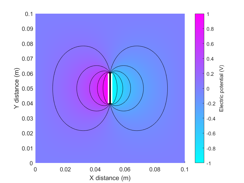
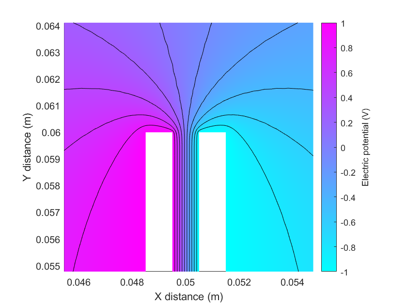
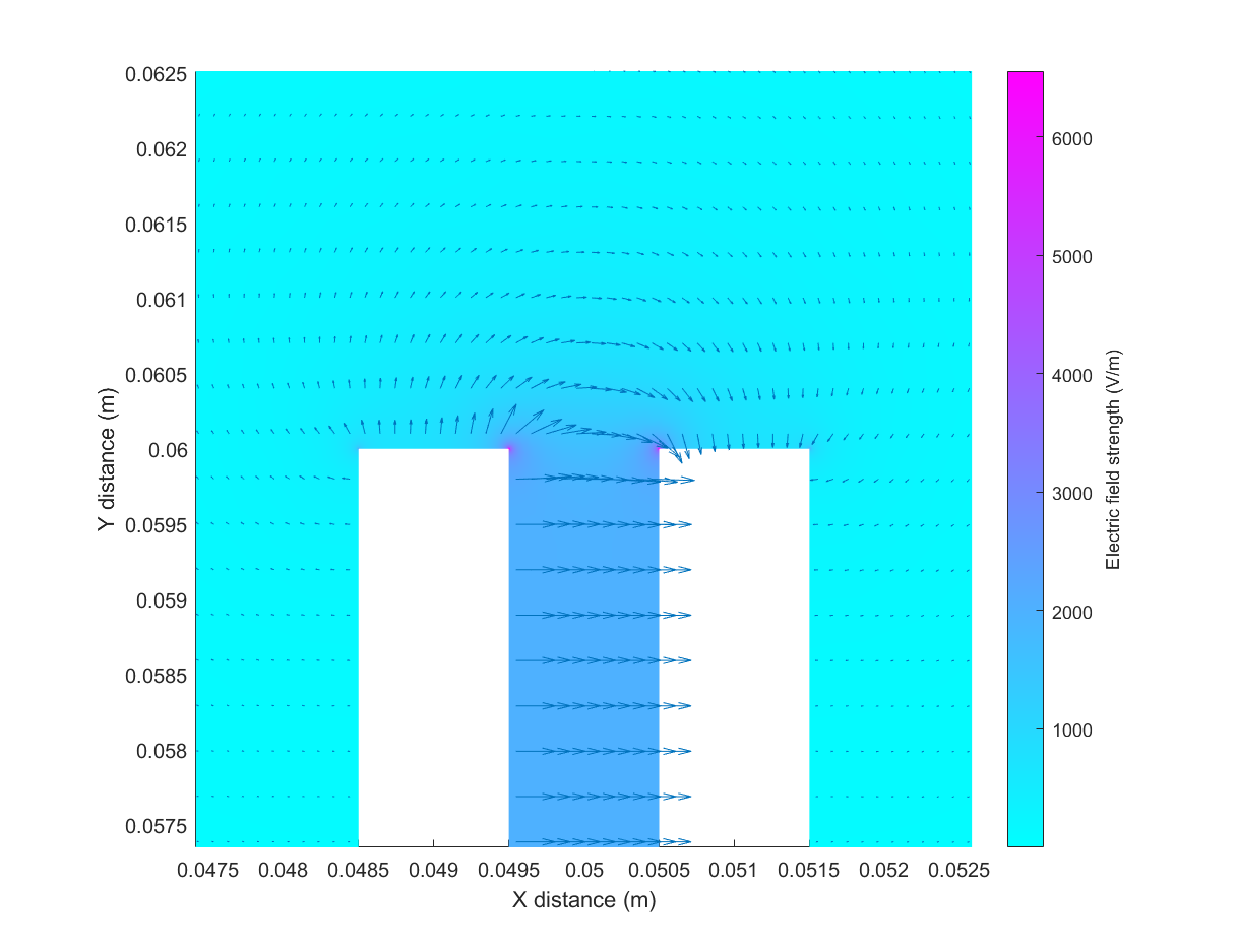
As shown in Figure 4, the electric field lines curve outwards near the edge of the capacitor. If this system were a sensor, and our goal was to measure changes in capacitance, these fringing effects may cause interference. For sensing purposes, we can minimise the edge effects by using guard plates (Figure 5).

Using these guard electrodes, the capacitance between the middle electrodes is closer to the ideal geometric value, $C=\epsilon A/d$.

Mechanisms of capacitance sensing

Using the equation $C=\epsilon A/d$ we can identify three ways that capacitance can vary:

1. Changes in area (e.g. by moving the electrodes sideways so that the area of overlap varies); or
2. Changes in separation distance (e.g. by moving the electrodes closer together or further apart); or
3. Changes in permittivity (e.g. by changing the properties of the material between the plates).

When we consider also the equivalent circuit of multiple capacitors, we can identify another mechanism:

4. Introducing or removing nearby objects that are capacitively coupled to the sensor, thereby adding or removing a capacitors from the equivalent circuit of the sensor.

Some mechanisms are shown in Figure 6.

Capacitive humidity sensors

Capacitance is a useful mechanism to detect water because water has a high permittivity. (This is because water molecules are polar, and can easily orient themselves in response to an applied electric field.) The relative permittivity of air is $\epsilon_{r}\approx1$ while for water it varies from $\epsilon_{r}=88$ at 0 °C to $\epsilon_{r}=55$ at 100 °C. Hence, adding water into the dielectric medium produces noticeable changes in permittivity.

A typical mechanism is to use some absorbent material that takes up moisture from the air. A properly chosen absorbent polymer film can be used to create an almost linear relationship between capacitance and relative humidity. However, the permittivity varies with temperature, so the temperature must also be measured and corrections applied.

Capacitive level sensors

Capacitance can be used to measure the level of liquid, as shown in Figure 7.

The electrodes may have various geometries, for example, they may be cylindrical with an inner electrode and an outer electrode where the liquid travels up the middle like a pipe. Alternatively they may have flat electrodes arranged as parallel plates or coplanar plates. If the electrodes are inside the liquid, then they must be covered with an insulating material. Alternatively, the electrodes may be placed on the outside of the container walls.

Since the air and liquid have different permittivity values, the capacitance per unit length in the air and liquid region are different. As the water level rises, the proportion of the capacitor with a high permittivity increases, resulting in a close to linear increase in capacitance.

Again there is a temperature dependence that must be accounted for. One strategy to do this is to include two more electrode pairs to measure the capacitance of the liquid and air. This can be used to correct for changes in temperature.

Other applications

• Capacitance can be used to measure small displacements by moving the electrodes with respect to each other. For example some accelerometers measure the deflection of a proof mass suspended on a miniature spring.
• Studio condenser microphones measure the deflection of a diaphragm through change in capacitance.
• An electrically conducting object can be used as one electrode in a single ended capacitance probe.

Capacitive interface circuits

Interface circuits for capacitive sensors often use a sinusoidal voltage or current. In this case, the capacitive sensor can be represented by a complex impedance $Z=R-jX$ where $R$ is a (typically undesirable) series resistance and $X=\frac{1}{\omega C}$ is the reactance of the sensor. Note $\omega=2\pi f$ where $f$ is the frequency of the AC power source.

For some intuition, consider a capacitance sensor with $C=100$ pF. An AC excitation frequency of 10 kHz would give $X=160$ kΩ, whereas an excitation frequency of 100 MHz would give $X=16$ Ω. These reactances could be measured using 2-wire or 4-wire measurement circuits, just as for resistance sensors. Simply use a sinusoidal source and measure the RMS voltage and current, and find the impedance with Ohm’s law.

However, there are also various circuit designs that are more specialised to capacitive sensor interfacing.

The auto-balancing bridge

The auto-balancing bridge (Figure 8) is a simple circuit that is common in LCR meters. To understand this circuit, notice that the op-amp creates a virtual ground at $V_m$. Therefore $i_C$ is completely determined by the voltage source and capacitor. However, all the current $i_C$ must flow through the resistor, creating a voltage at the output $V_o$. Therefore by measuring $V_o$, it is simple to calculate the capacitance.

Op-amp circuits with linear responses

When impedance is linearly proportional to the measurand

Consider a capacitive sensor where the separation distance is varied. Specifically, consider that the distance is given by

where $d_0$ is a typical distance and $x$ represents the influence of the measurand. In this case the sensor response is of the form:

where $C_0$ is the capacitance at $x=0$.

Now consider the impedance of this capacitive sensor:

Notice that impedance is linearly proportional to the measurand. A suitable interface circuit is shown in Figure 9.

The resistor $R$ is necessary to provide feedback at DC. The AC behaviour of this circuit is that of an inverting amplifier, i.e.

where $Z_{x}=1/(j\omega C_{x})$ is the impedance of the sensor and $Z=1/(j\omega C)$ is the impedance of the fixed capacitor $C$. If we choose $R\gg\left|Z_{x}\right|$ then $Z_{x}||R\approx Z_{x}$ and the output voltage becomes

Notice that the output is linear with respect to $x$.

When impedance is inversely proportional to the measurand

Other types of capacitive sensors may have variations in permittivity or surface area, i.e. a response of the form:

In this case the capacitor’s impedance is

i.e. impedance is inversely proportional to the measurand. In this case, swap the placement of the variable and fixed capacitors:

The resulting output voltage is

Again notice that the output voltage is linearly proportional to $x$.

AC bridges

Bridge circuits can also be used for capacitive sensors, as shown in Figure 11.

The analysis is similar to the Wheatstone bridge except that impedances are used instead of resistances.

A variation of this concept is the Blumlein bridge, where a centre-tapped transformer is used on one side (Figure 12).

The advantage of this design is that the sensing side has galvanic isolation from the excitation source, so that it can be separately grounded. Notice that $V_{0}$ is a single ended voltage with respect to the indicated ground.

To analyse this circuit, notice that the action of the transformer is to produce a voltage source with magnitude $nV_{i}$ where $n$ is the turns ratio. Using a voltage divider formula and recognising that the halfway point of the centre-tapped transformer has half the voltage, we can write the output voltage as:

Circuits based on charging & discharging capacitors

Transformers cannot be miniaturised, hence other interfacing circuits have been developed for integrated circuits. Instead of using sinusoidal excitation, capacitance can also be measured based on its charging and discharging behaviour.

Charge transfer

Charge can be transferred from an unknown capacitor to a known capacitor (Figure 13).

This circuit operates in three steps:

1. The unknown capacitor $C_{x}$ is charged to a fixed voltage $V_{r}$.
2. The energy stored in $C_{x}$ is shared with $C_{1}$ by opening S1 and closing S2. The output voltage $V_{0}$ can then be measured.
3. $C_{1}$ is discharged by closing S3, and the process repeats.

The output voltage can be derived by conservation of charge. You will show in tutorial questions that

$C_{x}$ can then be calculated from this equation.

Variable frequency oscillators

An oscillator is a circuit that produces a periodic waveform. A common strategy to measure capacitance is to design an oscillator circuit whose output frequency depends upon the capacitance of the sensor. An example is the relaxation oscillator that uses a comparator:

The sensor can be either $C$ or $R$. The oscillation period is proportional to the $RC$ time constant of the circuit, so changes in either $R$ or $C$ will change the oscillation frequency. In this design, the output voltage $V_{0}$ is a square wave, the frequency of which can be monitored using a microcontroller.

As drawn, this circuit is for a comparator with push-pull outputs, for example the TLV3491. The pullup resistor $R_{p}$ is necessary to make this circuit work with a single power rail. This circuit is suitable for oscillations up to tens of kHz, which limits the range of capacitances that can be measured.

Other types of oscillators (e.g. Wein bridge oscillators, Hartley oscillators, and Colpitts oscillators) operate at higher frequencies, and hence can be used with sensors whose capacitance is smaller. The principle is the same: changes in capacitance cause changes in oscillation frequency, and the frequency is then measured with a microcontroller or other digital circuit.

Conclusion

Capacitance is commonly used for sensing purposes because it enables relatively long range, contactless measurements. The most famous example of capacitive sensing is the touchscreen found in many portable electronics devices. Capacitance is also common for sensing the presence or absence of various materials, for humidity sensing, and more.

There are two main types of interface circuits for capacitive sensors. In many designs, an AC voltage source is used to treat the capacitance as a complex impedance, and the impedance measured using similar methods to that of resistive sensors. In other designs, changes in capacitance control the timing of an oscillator or the time constant of an RC circuit.

References

Ramon Pallas-Areny and John G. Webster, Sensors and Signal Conditioning, 2nd edition, Wiley, 2001.

Winncy Y. Du, Resistive, Capacitive, Inductive, and Magnetic Sensor Technologies, CRC Press, 2015.